Instrumenting a Subsea Desalination Prototype at 1,000 Feet

In 2020 I was part of a small team building a proof-of-concept desalination system designed to run fully submerged in the ocean, roughly 1,000 feet down. I wasn’t responsible for the desalination hardware itself — the reverse-osmosis membranes, high-pressure pump, and valve manifold belonged to someone else’s expertise. My job was the sensor side: getting water pressure, flow, and depth readings off the module and up the umbilical to where people could actually see them.

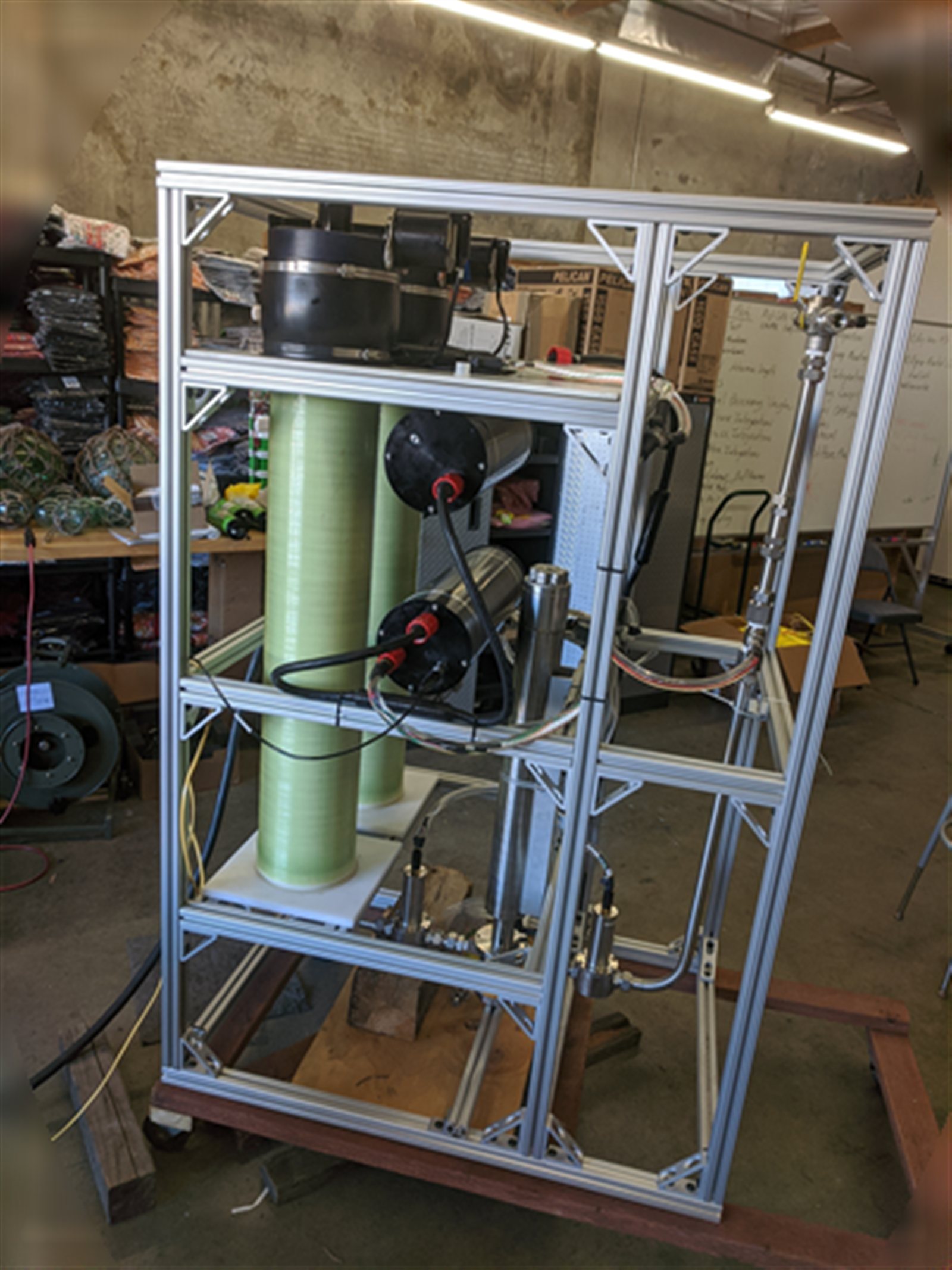
The module mid-assembly — this is early enough that the depth sensor and umbilical hadn't gone on yet.

The module

The frame in the photo above is the whole rig: two long membrane housings, a plumbing manifold carrying the flow meter and pressure sensors, and two black pressure vessels — sealed housings rated for the ambient pressure at depth. The Raspberry Pi and sensor interface this post is actually about lived inside the lower one. None of the desalination hardware itself was mine to design; My job was to connect to the sensors and get their readings topside.

Sensor interface

Reading those sensors and getting the data topside came down to a Raspberry Pi 3 Model B — sealed inside that pressure vessel on the module itself — paired with a small stack of COTS and custom hardware:

• A 16-bit I2C ADC breakout (an ADS1115-based COTS Gravity module) reading the two pressure sensors — one of them through a resistor divider to bring its output into the ADC’s input range — plus a second board at I2C address 0x49 reading a 4–20mA current-loop board.
• A GPIO-based pulse counter for the flow meter — an interrupt handler counted rising edges and turned the running count into a rate.
• A dedicated RS-232 link to a Paroscientific digital pressure sensor for depth, running on its own serial thread rather than sharing the I2C bus with everything else.

The sensor interface board mid-assembly.

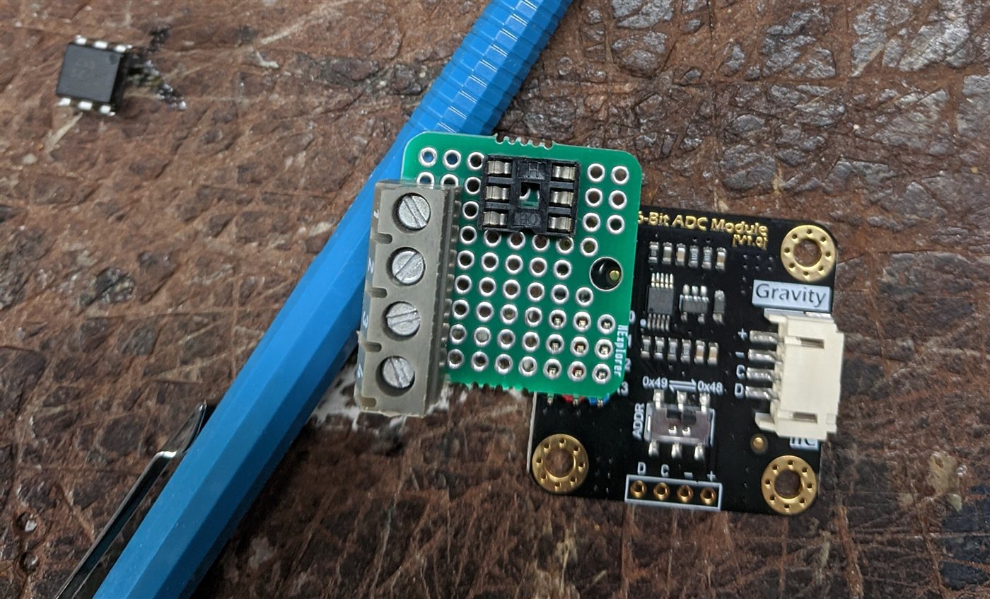
It needed to be built to survive the module’s testing phases — engineering test, final acceptance test, and customer test — sealed inside a pressure vessel.

Isolating and level-shifting the inputs

The schematic below is how each raw sensor signal gets conditioned before the Pi ever sees it. The flow meter’s pulse output runs through a 4N25 optocoupler, sketched out on graph paper before it ever touched a breadboard, which does two jobs at once: it scales the pulse down to the Pi’s GPIO logic level, and it isolates the Pi from whatever’s happening on the sensor side of that connector, so a wiring fault or a stray voltage out there can’t take out the single-board computer running the whole acquisition loop. The isolated pulse train lands on a GPIO input configured as an interrupt-driven counter. The pressure side needed its own bit of conditioning too — the resistor divider mentioned above, scaling one sensor’s output into the ADC’s input range.

The interface schematic: the 4N25 opto-isolator scales and isolates the flow signal for the Pi's GPIO, while a resistor divider conditions one of the two pressure sensors for the ADC.

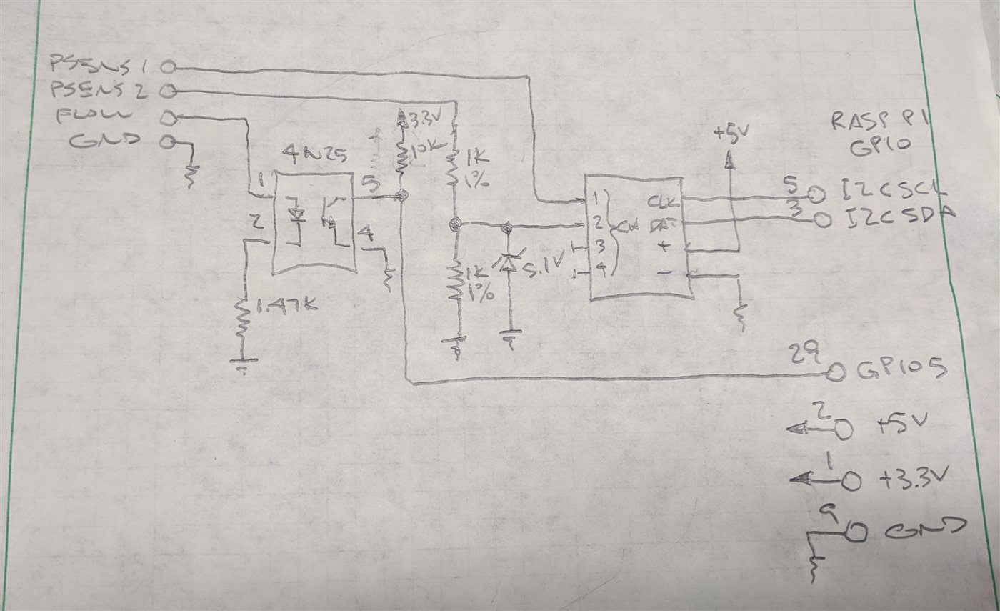
Hand-drawn and debuggable with a multimeter — there was no reason to make this a PCB for a proof-of-concept that would run once, log data, and get pulled back out of the water.

Simulating before soldering

Before committing the isolation stage to a breadboard, I modeled it in LTSpice: a pulse train standing in for the flow meter’s output, driving the 4N25 through its input resistor and into the pull-up network on the output side. The point wasn’t to prove the concept — opto-isolators are well-understood parts — it was to confirm the RC time constant of that pull-up network didn’t round the edges off enough to confuse the Pi’s interrupt handler at the flow rates I expected to see.

LTSpice model of the opto-isolator stage — the isolated output (green) tracks the drive pulses (blue) cleanly enough for the Pi's interrupt handler to trust.

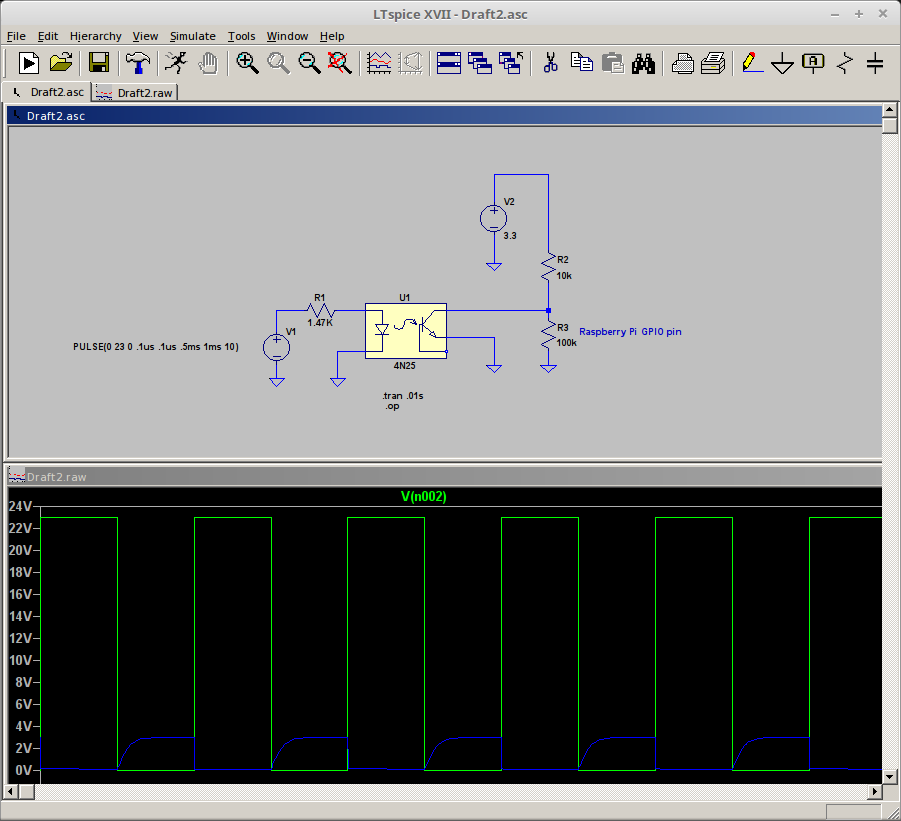
Good enough to trust the real hardware before it went anywhere near the water.

Depth on its own link

Depth came from the Paroscientific sensor over a plain RS-232 connection — simpler than the ADC/opto path everything else went through, and deliberately separate from it. A background thread configured the sensor for continuous sampling at 8Hz in its “Fetch Mode,” then read its comma-delimited output line by line as it arrived. Giving depth its own thread and its own wire meant a hiccup on the pressure/flow side couldn’t stall the one measurement everybody cared about most.

From sensors to CSV

Everything else ran off a 100-millisecond timer — 10Hz — that pulled the latest pressure, current-loop, and depth readings into a single CSV record:

#define INTERVAL 100    // 10Hz sample freq

void readSens()
{
    ...
    p1 = readAdc(0);
    p2 = readAdc(1);
    ...
    getParo(pp, pt);              // latest depth/temp from the serial thread

    sprintf(buf, "%ld.%03d, %4.3f, %4.3f, %.1lf, %.1lf, %.3lf, ...\n",
        t, getMsec(), p1, p2, f1, pp, pt, t1, t2, cs, tp1, tp2);

    fprintf(fp, "%s", buf);       // write record to logfile
    fflush(fp);

    if (t != lastTime)            // dump record to UDP port at 1Hz
    {
        sendStr(buf);
        lastTime = t;
    }
}

Every record got written to a local logfile and echoed to the console, so anyone standing next to the Pi could tell it was alive. Once a second, the same record went out over UDP broadcast on the local network for the topside laptop to pick up — the 10Hz logfile was the record of truth, the 1Hz broadcast was just enough to watch things happen live.

Topside: logging and a live dashboard

On the surface, a Windows laptop listened on that UDP port and logged everything to disk for later analysis in Excel or MATLAB. That logfile was the deliverable — but a file on disk doesn’t tell you anything is wrong until you go looking, and scrolling CSV isn’t the same as knowing your depth reading just flatlined mid-run. I built a small LabVIEW dashboard to put the numbers in front of whoever was running the test, updating live as records came in: depth in meters of seawater, flow in gallons per minute, and two pressure channels — a low-range and a high-range gauge, each paired with a strip chart.

The LabVIEW front panel: depth, flow, and two pressure channels, each with a live strip chart alongside the numeric readout.

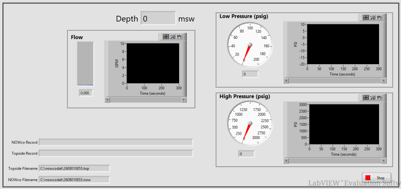
Behind that front panel is a single UDP receive loop: unpack the incoming CSV record, apply a per-channel zero-offset, and route each value to its gauge, chart, and file record — one loop, no polling, updating exactly as fast as data arrived from the module.

The block diagram behind the front panel — one UDP receive loop unpacking, scaling, and routing each channel.

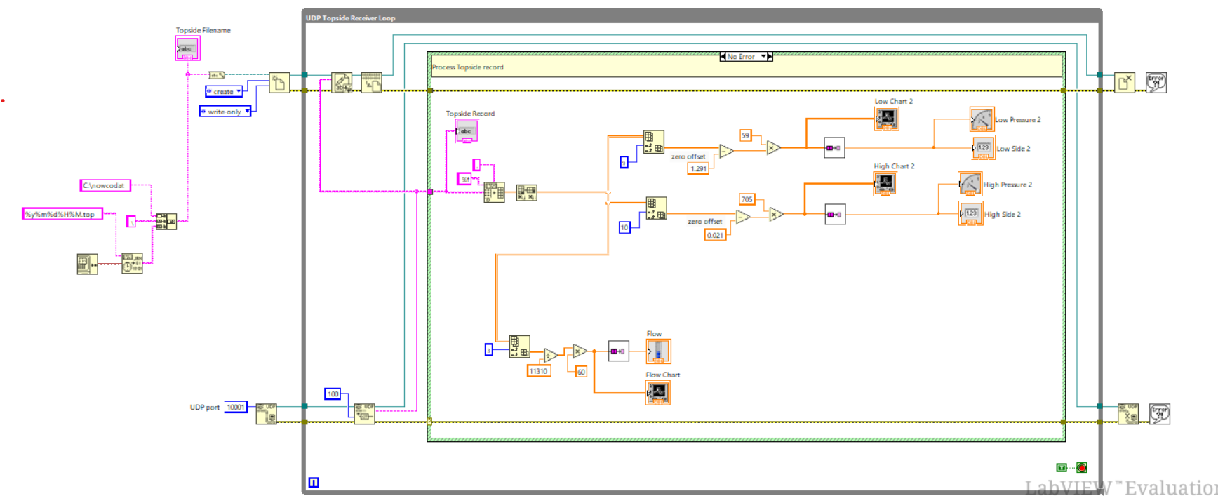
Nothing about the dashboard changed what got logged; the Windows laptop wrote the record of truth to disk exactly the same either way. What the dashboard bought was confidence during the run itself — a bad connector or a sensor that stopped responding showed up as a flat line on screen instead of a bad surprise days later in a spreadsheet.

Takeaways

• Isolate anything that leaves the board. A 4N25 optocoupler between the sensor wiring and the Pi’s 5V logic meant a flaky field connection couldn’t take out the single-board computer running the whole acquisition loop.
• Simulate the boundary stage, not just the fun part. The LTSpice check wasn’t about proving an optocoupler works — it was about catching edge-rounding on paper instead of on the bench.
• Give the measurement you care about most its own path. Depth ran on a dedicated serial thread, separate from the shared I2C/ADC loop, so a hiccup on one side couldn’t stall the other.
• Logging isn’t the same as visibility. The topside laptop was already writing every record to disk for later analysis — the dashboard didn’t change that. What it added was letting someone watching the run catch a problem while it was still happening, not days later in a spreadsheet.